k-최근접 이웃 - 기계학습과 대화

k-최근접 이웃(k-Nearest Neighbors, kNN) 은 가장 기본적인 기계학습 알고리즘 중 하나입니다. 경험한 데이터를 그대로 저장해 두었다가, 새로운 데이터가 들어오면 저장된 데이터 중 가장 가까운 이웃을 찾아 그 이웃의 값으로 예측합니다. 별도의 모델(매개변수)을 학습하지 않고 데이터 자체를 기억하므로 비매개변수(non-parametric) 알고리즘으로 분류됩니다.

예를 들어 두 유형으로 나뉜 데이터에서 새 데이터가 한쪽 유형의 점들에 가까우면 그 유형으로 분류합니다. 분류와 회귀 모두에 사용할 수 있습니다.

import numpy as np
import pandas as pd
import matplotlib.pyplot as plt
import sklearn

print(f'scikit-learn: {sklearn.__version__}')

scikit-learn: 1.1.1

1데이터 적재¶

붓꽃 데이터를 적재합니다. 특성 X와 목표값 y로 나누어 가져옵니다.

from sklearn.datasets import load_iris

iris_bunch = load_iris()
iris = pd.DataFrame(iris_bunch.data, columns=iris_bunch.feature_names)
iris['label'] = pd.Series(iris_bunch.target).replace(np.unique(iris_bunch.target), iris_bunch.target_names)
iris[:5]

X, y = load_iris(as_frame=True, return_X_y=True)

X[:3]

y.value_counts()

0    50
1    50
2    50
Name: target, dtype: int64

유형별색상 = iris.target.replace({0:'red', 1:'green', 2:'blue'})
iris.frame.plot(kind='scatter', x='x1', y='x3', c=유형별색상)

X_new = np.array([[5.5, 2.0], [5.8, 4.8]])
plt.scatter(X_new[:, 0], X_new[:, 1], color='black', marker='x')

2거리 측정¶

최근접 이웃을 찾으려면 두 데이터 사이의 거리를 정의해야 합니다. 가장 널리 쓰이는 것은 유클리드 거리로, 각 차원의 차이를 제곱해 더한 뒤 제곱근을 취합니다 — 두 점을 잇는 직선 거리입니다. 절대값의 합으로 계산하는 맨해튼 거리도 있으며, 둘 다 민코프스키 거리의 특수한 경우입니다.

여러 특성의 단위가 서로 다르면 큰 값이 거리를 지배할 수 있으므로, 거리 기반 알고리즘에서는 단위 변환(정규화)이 중요합니다.

벡터거리산출 = lambda xi, xj: np.sqrt(np.sum((xi - xj) ** 2))

def 최근접이웃분류기(훈련데이터, 입력데이터, 이웃수=1):
    Xs, y = 훈련데이터
    xi = 입력데이터
    이웃거리 = []
    for xj in Xs:
        이웃거리.append(벡터거리산출(xi, xj))
    
    거리순_이웃색인 = np.argsort(이웃거리)
    최근접이웃 = 거리순_이웃색인[:이웃수]
    이웃라벨 = y[최근접이웃]
    if len(이웃라벨) > 1:
        예측 = pd.Series(이웃라벨).value_counts().index[0]
    else:
        예측 = 이웃라벨[0]
    print(f'xi={xi} -> kNN(k={이웃수}) -> y_pred={예측}')
    return 예측

Xs = iris.data.to_numpy()[:, [0, 2]]
y = iris.target.to_numpy()

최근접이웃분류기(훈련데이터=(Xs, y), 입력데이터=X_new[0])
최근접이웃분류기(훈련데이터=(Xs, y), 입력데이터=X_new[1], 이웃수=1)
최근접이웃분류기(훈련데이터=(Xs, y), 입력데이터=X_new[1], 이웃수=4)

3분류¶

kNN으로 붓꽃 품종을 분류해 보겠습니다. 새 데이터의 최근접 이웃들을 찾은 뒤, 이웃들의 다수결로 유형을 결정합니다.

from sklearn.model_selection import train_test_split

X_train, X_test, y_train, y_test = train_test_split(X, y, stratify=y, random_state=0)

from sklearn.neighbors import KNeighborsClassifier

붓꽃분류기 = KNeighborsClassifier(n_neighbors=1)
붓꽃분류기.fit(X_train, y_train)
붓꽃분류기.score(X_test, y_test)

0.9736842105263158

from sklearn.neighbors import KNeighborsClassifier

붓꽃분류기 = KNeighborsClassifier(n_neighbors=5)
붓꽃분류기.fit(X_train, y_train)
붓꽃분류기.score(X_test, y_test)

1.0

X_train, X_test, y_train, y_test = train_test_split(X, y, stratify=y, random_state=1)

from sklearn.neighbors import KNeighborsClassifier

붓꽃분류기 = KNeighborsClassifier(n_neighbors=1)
붓꽃분류기.fit(X_train, y_train)
붓꽃분류기.score(X_test, y_test)

0.9736842105263158

from sklearn.neighbors import KNeighborsClassifier

붓꽃분류기 = KNeighborsClassifier(n_neighbors=5)
붓꽃분류기.fit(X_train, y_train)
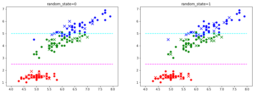
붓꽃분류기.score(X_test, y_test)

0.9473684210526315

예측 결과 분석

random_state=0

시험 데이터가 쉬움

random_state=1

보다 어려운 데이터가 포함됨

특성목록 = X.columns
x1 = 특성목록[0]
x3 = 특성목록[2]
print(f'선택한 특성들: {x1}, {x3}')

유형별_색상사전 = dict(zip(np.unique(y), ['red', 'green', 'blue']))

_, subplots = plt.subplots(1, 2, figsize=(15, 5))

def plot(ax, title):
    ax.set_title(title)
    ax.scatter(X_train[x1], X_train[x3], c=y_train.replace(유형별_색상사전))
    ax.scatter(X_test[x1], X_test[x3], marker='x', s=80, c=y_test.replace(유형별_색상사전))
    # 유형 경계
    ax.hlines(2.5, xmin=4, xmax=8, colors='magenta', linestyle='--')
    ax.hlines(5.0, xmin=4, xmax=8, colors='cyan', linestyle='--')

X_train, X_test, y_train, y_test = train_test_split(X, y, stratify=y, random_state=0)
plot(subplots[0], 'random_state=0')
    
X_train, X_test, y_train, y_test = train_test_split(X, y, stratify=y, random_state=1)
plot(subplots[1], 'random_state=1')

선택한 특성들: sepal length (cm), petal length (cm)

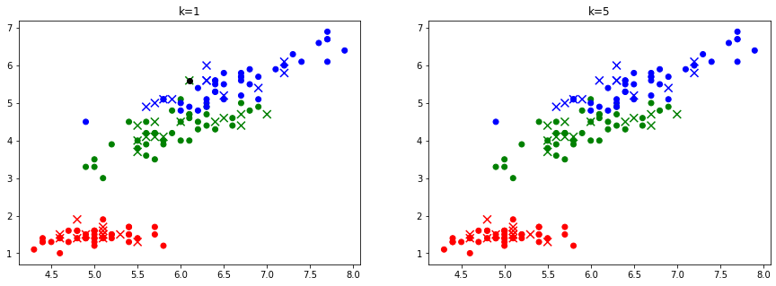
3.1이웃 수 설정¶

이웃 수 $k$ 는 kNN의 핵심 설정입니다. $k=1$ 은 가장 가까운 한 이웃만 보는데, 특정 표본에 과도하게 민감해 대개 바람직하지 않습니다. 보통 둘 이상의 이웃을 다수결에 사용하며, 동점을 피하려고 홀수로 두는 경우가 많습니다. $k$ 를 임의로 정할 수 있어 'k-최근접 이웃’이라 부릅니다.

# 이웃수에 따른 예측 결과
def 결과출력(ax, title):
    print(f'이웃수 {이웃수}: {붓꽃분류기.score(X_test, y_test):.2%}')
    y_pred = 붓꽃분류기.predict(X_test)
    오답표본 = X_test.loc[y_test != y_pred]
    
    ax.set_title(title)
    ax.scatter(X_train[x1], X_train[x3], c=y_train.replace(유형별_색상사전))
    ax.scatter(X_test[x1], X_test[x3], marker='x', s=80, c=pd.Series(y_pred).replace(유형별_색상사전))
    ax.scatter(오답표본[x1], 오답표본[x3], c='black')

_, subplots = plt.subplots(1, 2, figsize=(15, 5))

X_train, X_test, y_train, y_test = train_test_split(X, y, stratify=y, random_state=0)

이웃수 = 1
붓꽃분류기 = KNeighborsClassifier(n_neighbors=이웃수).fit(X_train, y_train)
결과출력(subplots[0], 'k=1')

이웃수 = 5
붓꽃분류기 = KNeighborsClassifier(n_neighbors=이웃수).fit(X_train, y_train)
결과출력(subplots[1], 'k=5')

이웃수 1: 97.37%
이웃수 5: 100.00%

X_train, X_test, y_train, y_test = train_test_split(X, y, stratify=y, random_state=6)

훈련결과 = {}
for 이웃수 in range(1, 11):
    붓꽃분류기 = KNeighborsClassifier(n_neighbors=이웃수)
    붓꽃분류기.fit(X_train, y_train)
    훈련점수 = 붓꽃분류기.score(X_train, y_train)
    시험점수 = 붓꽃분류기.score(X_test, y_test)
    훈련결과[이웃수] = {'train': 훈련점수, 'test': 시험점수}
    
pd.DataFrame(훈련결과).T.plot()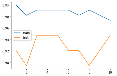

from sklearn.model_selection import train_test_split

def 모델평가(model, X, y, **설정):
    X_train, X_test, y_train, y_test = train_test_split(X, y, **설정)
    model.fit(X_train, y_train)
    훈련점수 = model.score(X_train, y_train)
    시험점수 = model.score(X_test, y_test)
    return {'train': 훈련점수, 'test': 시험점수}

훈련결과 = {}
for 이웃수 in range(1, 11):
    붓꽃분류기 = KNeighborsClassifier(n_neighbors=이웃수)    
    훈련결과[이웃수] = 모델평가(붓꽃분류기, X, y, stratify=y, random_state=6)
    
pd.DataFrame(훈련결과).T.plot()

붓꽃분류기.n_neighbors

10

붓꽃분류기 = KNeighborsClassifier(n_neighbors=5)
평가결과 = 모델평가(붓꽃분류기, X, y, stratify=y, random_state=6)
print('훈련점수: {train:.2%}, 시험점수: {test:.2%}'.format(**평가결과))
y_pred = 붓꽃분류기.predict(X_test)
y_pred[:5]

훈련점수: 99.11%, 시험점수: 94.74%

array([0, 2, 2, 0, 1])

붓꽃분류기.n_samples_fit_

112

훈련안된모델 = KNeighborsClassifier()
try:
    훈련안된모델.n_samples_fit_
except AttributeError as err:
    print(err)

'KNeighborsClassifier' object has no attribute 'n_samples_fit_'

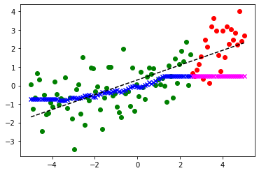
4회귀¶

kNN은 회귀에도 사용할 수 있습니다. 분류가 이웃들의 다수결이라면, 회귀는 최근접 이웃들의 값을 평균해 예측합니다.

x = np.linspace(-5., 5, 100)
random = np.random.RandomState(0)
noise = random.randn(len(x))
y = 0.4 * x + 0.3 + noise
plt.scatter(x, y)
plt.plot(x, y - noise, 'k--')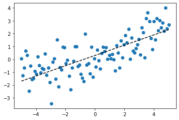

X = x.reshape(x.shape[0], 1)
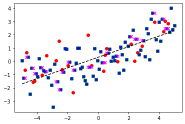
X_train, X_test, y_train, y_test = train_test_split(X, y, random_state=0)

from sklearn.neighbors import KNeighborsRegressor
from sklearn.metrics import r2_score

kreg = KNeighborsRegressor(n_neighbors=1).fit(X_train, y_train)
y_train_pred = kreg.predict(X_train)
y_test_pred = kreg.predict(X_test)

훈련점수 = r2_score(y_train, y_train_pred)
시험점수 = r2_score(y_test, y_test_pred)
assert 훈련점수 == kreg.score(X_train, y_train)
assert 시험점수 == kreg.score(X_test, y_test)

print(f'이웃수={kreg.n_neighbors} 훈련점수: {훈련점수:.3f}, 시험점수: {시험점수:.3f}')

plt.plot(x, y - noise, 'k--')
plt.scatter(X_train, y_train, color='green')
plt.scatter(X_test, y_test, color='red')
# 예측
plt.scatter(X_train, y_train_pred, color='blue', marker='x')
plt.scatter(X_test, y_test_pred, color='magenta', marker='x')

이웃수=1 훈련점수: 1.000, 시험점수: 0.288

훈련결과 = {}
for 이웃수 in range(1, 31):
    kreg = KNeighborsRegressor(n_neighbors=이웃수)
    훈련결과[이웃수] = 모델평가(kreg, X, y, random_state=0)
    
pd.DataFrame(훈련결과).T.plot()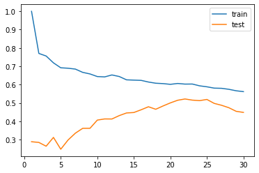

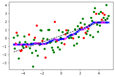
from sklearn.neighbors import KNeighborsRegressor
from sklearn.metrics import r2_score

kreg = KNeighborsRegressor(n_neighbors=25).fit(X_train, y_train)
y_train_pred = kreg.predict(X_train)
y_test_pred = kreg.predict(X_test)

훈련점수 = r2_score(y_train, y_train_pred)
시험점수 = r2_score(y_test, y_test_pred)
assert 훈련점수 == kreg.score(X_train, y_train)
assert 시험점수 == kreg.score(X_test, y_test)

print(f'이웃수={kreg.n_neighbors} 훈련점수: {훈련점수:.3f}, 시험점수: {시험점수:.3f}')

plt.plot(x, y - noise, 'k--')
plt.scatter(X_train, y_train, color='green')
plt.scatter(X_test, y_test, color='red')
# 예측
plt.scatter(X_train, y_train_pred, color='blue', marker='x')
plt.scatter(X_test, y_test_pred, color='magenta', marker='x')

이웃수=25 훈련점수: 0.588, 시험점수: 0.519

X_train, X_test, y_train, y_test = train_test_split(X, y, shuffle=False)

from sklearn.neighbors import KNeighborsRegressor
from sklearn.metrics import r2_score

kreg = KNeighborsRegressor(n_neighbors=25).fit(X_train, y_train)
y_train_pred = kreg.predict(X_train)
y_test_pred = kreg.predict(X_test)

훈련점수 = r2_score(y_train, y_train_pred)
시험점수 = r2_score(y_test, y_test_pred)
assert 훈련점수 == kreg.score(X_train, y_train)
assert 시험점수 == kreg.score(X_test, y_test)

print(f'이웃수={kreg.n_neighbors} 훈련점수: {훈련점수:.3f}, 시험점수: {시험점수:.3f}')

plt.plot(x, y - noise, 'k--')
plt.scatter(X_train, y_train, color='green')
plt.scatter(X_test, y_test, color='red')
# 예측
plt.scatter(X_train, y_train_pred, color='blue', marker='x')
plt.scatter(X_test, y_test_pred, color='magenta', marker='x')

이웃수=25 훈련점수: 0.227, 시험점수: -2.057