결정 트리(decision tree) 는 데이터를 여러 단계에 걸쳐 나누어 예측하는 알고리즘입니다. 마치 if/else 구문을 잇는 것처럼, 각 단계에서 특성 하나를 기준으로 데이터를 분기합니다. 선형 모델이 직선 하나로 나누기 어려운 비선형 분포도, 결정 트리는 분기를 거듭해 영역을 잘게 나누어 다룰 수 있습니다.
import numpy as np
import pandas as pd
import matplotlib.pyplot as plt
import sklearn

print(f'numpy: {np.__version__}')
print(f'pandas: {pd.__version__}')
print(f'scikit-learn: {sklearn.__version__}')
numpy: 2.2.6
pandas: 2.3.3
scikit-learn: 1.7.2
from sklearn.model_selection import train_test_split

def 모델평가(model, data, target, **설정):
    train_data, test_data, train_target, test_target = train_test_split(
        data, target, **설정)
    model.fit(train_data, train_target)
    scores = {
        'train': model.score(train_data, train_target),
        'test': model.score(test_data, test_target)
    }
    return pd.Series(scores)
1정보 엔트로피
결정트리가 특정한 분기를 할 때는, 무질서도 또는 불순도를 낮추기 위해 노력합니다. 여러 가지 가능성 중 더 나은 것을 선택하기 위해 정보를 정량적으로 평가합니다.
정보엔트로피산출 = lambda 확률: -np.sum(확률 * np.log2(확률 + 1e-9))
지니불순도산출 = lambda 확률: np.sum(확률 * (1 - 확률))
확률산출 = lambda labels: np.bincount(labels) / len(labels)

results = []
target = np.array([0, 1] * 4)
p = 확률산출(target)
results.append({
    'H': 정보엔트로피산출(확률산출(target)),
    'gini': 지니불순도산출(p),
    'p0': p[0], 'p1': p[1]
})
target = np.array([0, 1, 1, 1, 1, 1, 1, 0])
p = 확률산출(target)
results.append({
    'H': 정보엔트로피산출(확률산출(target)),
    'gini': 지니불순도산출(p),
    'p0': p[0], 'p1': p[1]
})
target = np.array([1] * 8)
p = 확률산출(target)
results.append({
    'H': 정보엔트로피산출(확률산출(target)),
    'gini': 지니불순도산출(p),
    'p0': p[0], 'p1': p[1]
})

pd.DataFrame(results).round(3)
Loading...
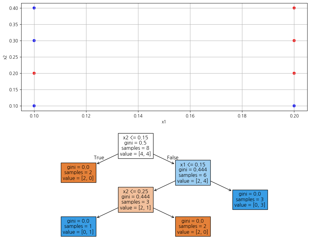
from sklearn.tree import DecisionTreeClassifier, plot_tree

x1 = np.array([0.1, 0.2])
x2 = np.array([0.1, 0.2, 0.3, 0.4])

X1, X2 = np.meshgrid(x1, x2)

data = np.stack([X1.ravel(), X2.ravel()]).T
target = np.array([0, 0, 1, 1, 0, 1, 0, 1])
print(pd.DataFrame(data, columns=['x1', 'x2']).assign(y=target))

tree = DecisionTreeClassifier(criterion='entropy') # 정보 엔트로피 (원조)
tree = DecisionTreeClassifier(criterion='gini') # 지니 불순도 (개선); 기본값
tree.fit(data, target)

plt.figure(figsize=(12, 10))
plt.subplot(2, 1, 1)
plt.scatter(X1, X2, c=target, cmap='bwr')
plt.xlabel('x1'); plt.ylabel('x2')
plt.grid()
plt.subplot(2, 1, 2)
plot_tree(tree, filled=True, feature_names=['x1', 'x2'])
plt.show()
x1 x2 y
0 0.1 0.1 0
1 0.2 0.1 0
2 0.1 0.2 1
3 0.2 0.2 1
4 0.1 0.3 0
5 0.2 0.3 1
6 0.1 0.4 0
7 0.2 0.4 1
from sklearn.datasets import make_classification
from sklearn.utils import Bunch
from sklearn.tree import DecisionTreeClassifier, plot_tree
_X, _y = make_classification(n_samples=400, n_features=10, n_informative=6,
n_redundant=2, random_state=0)
분류 = Bunch(data=_X, target=_y,
feature_names=[f'특성{i+1}' for i in range(10)],
target_names=['유형0', '유형1'])
print(분류.data.shape)
print(분류.target_names)
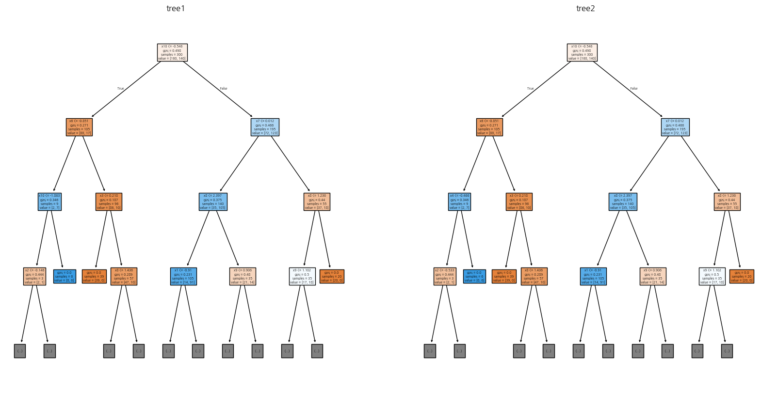
scores = {}
tree1 = DecisionTreeClassifier(random_state=0)
scores['tree1'] = 모델평가(tree1, 분류.data, 분류.target, random_state=3)
tree2 = DecisionTreeClassifier(random_state=1)
scores['tree2'] = 모델평가(tree2, 분류.data, 분류.target, random_state=3)
print(pd.DataFrame(scores).round(3))
출력설정 = {
'max_depth': 3,
'feature_names': [f'x{i+1}' for i in range(분류.data.shape[1])],
'filled': True,
}
plt.figure(figsize=(20, 10))
plt.subplot(1, 2, 1)
plot_tree(tree1, **출력설정); plt.title('tree1')
plt.subplot(1, 2, 2)
plot_tree(tree2, **출력설정); plt.title('tree2')
plt.show()(400, 10)
['유형0', '유형1']
tree1 tree2
train 1.00 1.00
test 0.83 0.87
from sklearn.tree import DecisionTreeClassifier, DecisionTreeRegressor, plot_treefrom sklearn.datasets import load_iris
iris = load_iris()
y = iris.target
X = iris.data[:, [0, 2]]
tree = DecisionTreeClassifier().fit(X, y)
tree.score(X, y)0.9933333333333333plt.figure(figsize=(10, 10))
_ = plot_tree(tree, feature_names=['x1', 'x3'])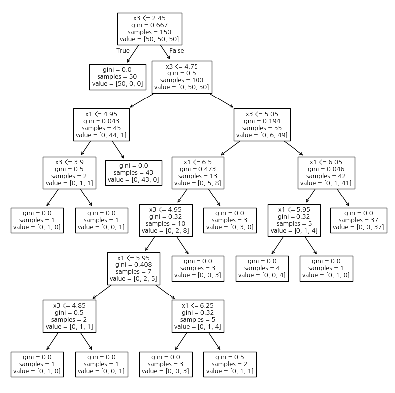
color_dict = dict(zip(np.unique(y), list('rgb')))
x1 = X[:, 0]
x3 = X[:, 1]
plt.scatter(x1, x3, c=pd.Series(y).replace(color_dict))
plt.hlines(2.45, x1.min(), x1.max())
plt.hlines(4.75, x1.min(), x1.max())
plt.vlines(4.95, x3.min(), 4.75)
plt.hlines(3.9, x1.min(), 4.95)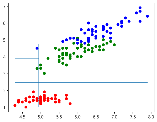
from sklearn.datasets import make_classification
from sklearn.utils import Bunch

_X, _y = make_classification(n_samples=400, n_features=10, n_informative=6,
                             n_redundant=2, random_state=0)
분류 = Bunch(data=_X, target=_y,
           feature_names=[f'특성{i+1}' for i in range(10)],
           target_names=['유형0', '유형1'])
from sklearn.tree import DecisionTreeClassifier
분류_tree = DecisionTreeClassifier()
display(모델평가(분류_tree, 분류.data, 분류.target, random_state=0))
print(f'최대 깊이: {분류_tree.get_depth()}')train 1.00
test 0.81
dtype: float64최대 깊이: 8
사전 가지치기 (pre-pruning)
1.1가지치기
결정 트리는 모든 이파리가 순수해질 때까지 분기하면 표현력이 최대가 되지만, 그만큼 훈련 데이터에 과적합되기 쉽습니다. 가지치기(pruning) 로 표현력을 규제해 과적합을 완화합니다. 가장 간단한 방법은 트리의 최대 깊이(max_depth) 를 제한하는 것으로, 순수 노드에 도달하기 전에 분기를 멈춰 훈련 정확도를 일부 희생하는 대신 일반화 성능을 높입니다.
분류_tree = DecisionTreeClassifier(max_depth=4)
display(모델평가(분류_tree, 분류.data, 분류.target, random_state=0))
print(f'최대 깊이: {분류_tree.get_depth()}')
train 0.886667
test 0.900000
dtype: float64최대 깊이: 4
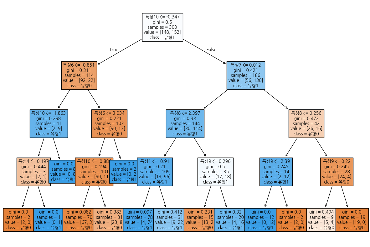
결정 트리 시각화
from sklearn.tree import plot_tree # version > 0.20

plt.figure(figsize=(15, 10))
_ = plot_tree(
    분류_tree, max_depth=4,
    feature_names=분류.feature_names, class_names=분류.target_names,
    fontsize=10, filled=True
)
특성 중요도 (feature importance)
pd.Series(분류_tree.feature_importances_, index=분류.feature_names).plot(kind='barh')<Axes: >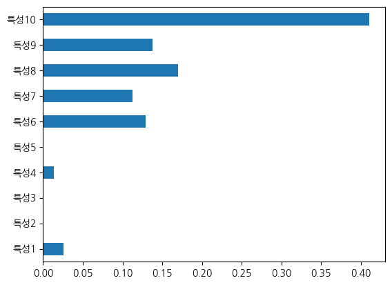
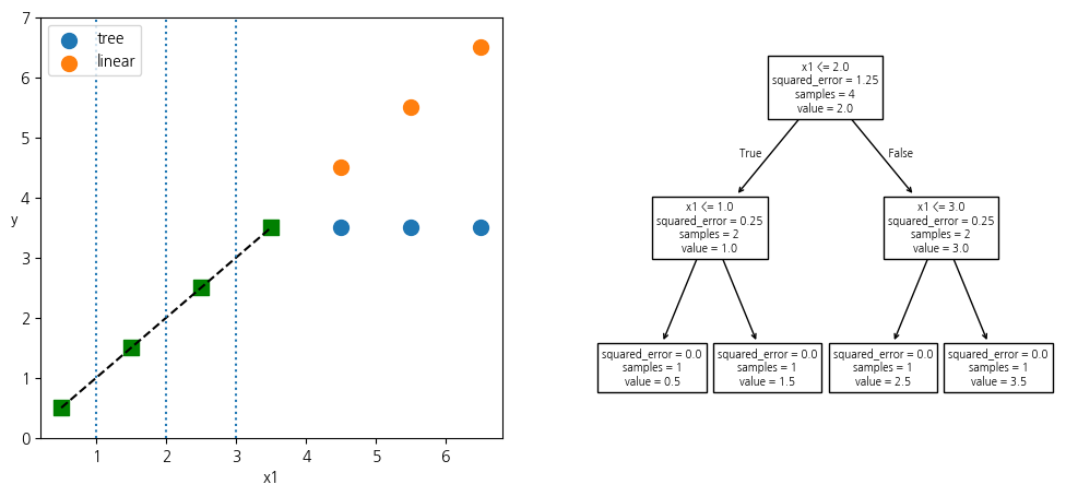
결정트리 외삽 문제
from sklearn.tree import DecisionTreeRegressor, plot_tree
from sklearn.linear_model import LinearRegression

xs = np.array([0.5, 1.5, 2.5, 3.5])
ys = xs

Xs = xs.reshape(-1, 1)
tree = DecisionTreeRegressor().fit(Xs, ys)
linear = LinearRegression().fit(Xs, ys)

X_new = np.array([[4.5, 5.5, 6.5]]).T

plt.figure(figsize=(12, 5))
plt.subplot(121)
plt.plot(xs, ys, 'k--')
plt.scatter(xs, ys, s=100, c='g', marker='s')
# 결정트리 영역 표시
plt.vlines([1.0, 2.0, 3.0], 0, 7, linestyles='dotted')
# 결정트리 예측
plt.scatter(X_new, tree.predict(X_new), s=100, label='tree')
# 선형회귀 예측
plt.scatter(X_new, linear.predict(X_new), s=100, label='linear')
plt.legend()
plt.ylim(0, 7)
plt.xlabel('x1')
plt.ylabel('y', rotation=0)
plt.subplot(122)
# 결정트리 그래프
plot_tree(tree, feature_names=['x1'])
plt.show()