PCA

import numpy as np
import pandas as pd
import matplotlib.pyplot as plt
import sklearn

import numpy as np
import matplotlib.pyplot as plt
from sklearn.decomposition import PCA
from sklearn.linear_model import LogisticRegression
from sklearn.tree import DecisionTreeClassifier

# Generate the x1 and x2 features
np.random.seed(42)
n_samples = 1000
x1 = np.random.rand(n_samples) * 10  # Values between 0 and 10
x2 = np.random.rand(n_samples) * 10  # Values between 0 and 10

# Apply the identity function
y_values = x1 + x2
# Set the threshold
threshold = 10
# Create binary target variable y based on the threshold
y = np.where(y_values >= threshold, 1, 0)

# Combine x1 and x2 into a single feature matrix X
X = np.column_stack((x1, x2))
X_pca = PCA(n_components=2).fit_transform(X)

# Fit a logistic regression model
model_1 = LogisticRegression().fit(X, y)
print(f'y1={model_1.coef_[0][0]:.2f} x1 + {model_1.coef_[0][1]:.2f} x2 + {model_1.intercept_[0]:.2f}')
print(model_1.score(X, y))
model_2 = LogisticRegression().fit(X_pca, y)
print(f'y2={model_2.coef_[0][0]:.2f} x1 + {model_2.coef_[0][1]:.2f} x2 + {model_2.intercept_[0]:.2f}')
print(model_2.score(X_pca, y))
model_3 = DecisionTreeClassifier().fit(X, y)
print(model_3.score(X, y))
print(model_3.get_depth())
model_4 = DecisionTreeClassifier().fit(X_pca, y)
print(model_4.score(X_pca, y))
print(model_4.get_depth())

z0 = lambda x1, w, b: (w[0] * x1 + b) / -w[1]

# Plot the dataset
plt.figure(figsize=(12, 6))
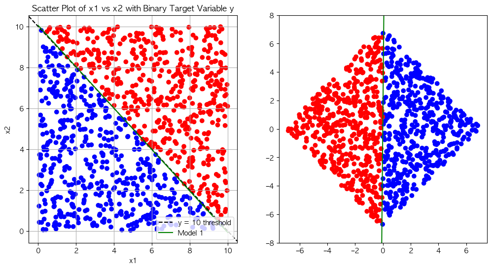
plt.subplot(121)
plt.scatter(X[:, 0], X[:, 1], c=y, cmap=plt.cm.bwr)
plt.axline((0, 10), slope=-1, color='black', linestyle='--', label='y = 10 threshold')
x1 = np.linspace(0, 10, 100)
plt.plot(x1, z0(x1, model_1.coef_[0], model_1.intercept_[0]), color='green', label='Model 1')
plt.xlabel('x1')
plt.ylabel('x2')
plt.title('Scatter Plot of x1 vs x2 with Binary Target Variable y')
plt.legend()
plt.grid(True)

plt.subplot(122)
plt.scatter(X_pca[:, 0], X_pca[:, 1], c=y, cmap=plt.cm.bwr)
x1_min = X_pca[:, 0].min()
x1_max = X_pca[:, 0].max()
x1 = np.linspace(x1_min,x1_max, 100)
plt.plot(x1, z0(x1, model_2.coef_[0], model_2.intercept_[0]), color='green', label='Model 1')
plt.ylim(-8, 8)
plt.show()

import numpy as np
import matplotlib.pyplot as plt
from sklearn.datasets import make_swiss_roll
from sklearn.decomposition import PCA

# Generate the Swiss Roll dataset
n_samples = 1000
noise = 0.05
X, color = make_swiss_roll(n_samples=n_samples, noise=noise)

# Plot the original Swiss Roll dataset
fig = plt.figure(figsize=(12, 6))
ax = fig.add_subplot(121, projection='3d')
ax.scatter(X[:, 0], X[:, 1], X[:, 2], c=color, cmap=plt.cm.Spectral)
ax.set_title("Original Swiss Roll in 3D")
ax.set_xlabel("X")
ax.set_ylabel("Y")
ax.set_zlabel("Z")

# Apply PCA to project the data to 2D
pca = PCA(n_components=2)
X_pca = pca.fit_transform(X)

# Plot the PCA-transformed data
ax = fig.add_subplot(122)
sc = ax.scatter(X_pca[:, 0], X_pca[:, 1], c=color, cmap=plt.cm.Spectral)
ax.set_title("PCA Projection of Swiss Roll to 2D")
ax.set_xlabel("Principal Component 1")
ax.set_ylabel("Principal Component 2")
plt.colorbar(sc)
plt.show()