캘리포니아 주택 가격 - 기계학습과 대화

캘리포니아 주택 가격 데이터로 회귀를 연습합니다. 여러 지역 특성(소득·방 수·위치 등)으로 주택 가격의 중앙값을 예측하는 문제입니다. 기본 선형 모델로 시작해, 단위 변환과 특성 공학(다항식·상호작용·구간 분할)으로 성능을 끌어올리는 과정을 살펴보겠습니다.

import numpy as np
import pandas as pd
import matplotlib.pyplot as plt
import sklearn

print('Scikit-Learn', sklearn.__version__)

Scikit-Learn 1.7.2

from sklearn.model_selection import train_test_split

def 모델평가(model, data, target, **설정):
    train_data, test_data, train_target, test_target = train_test_split(
        data, target, **설정)
    model.fit(train_data, train_target)
    scores = {
        'train': model.score(train_data, train_target),
        'test': model.score(test_data, test_target)
    }
    return pd.Series(scores)

from sklearn.datasets import fetch_california_housing

housing = fetch_california_housing(as_frame=True)
print(housing.data.shape)
print(housing.target.dtype) # 회귀 출력
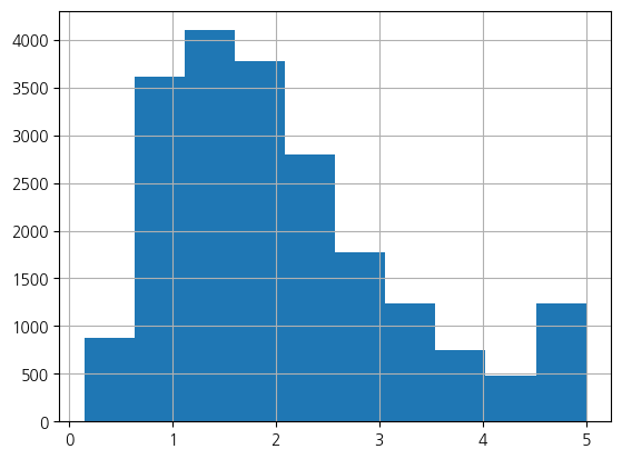
housing.target.hist()
plt.show()

(20640, 8)
float64

from sklearn.preprocessing import StandardScaler

scaler = StandardScaler()
scaled_data = scaler.fit_transform(housing.data)
# 평균이 0, 표준편차가 1인지 확인
assert np.allclose(scaled_data.mean(axis=0), 0) and \
    np.allclose(scaled_data.std(axis=0), 1)
pd.DataFrame(scaled_data, columns=housing.data.columns).boxplot()
plt.show()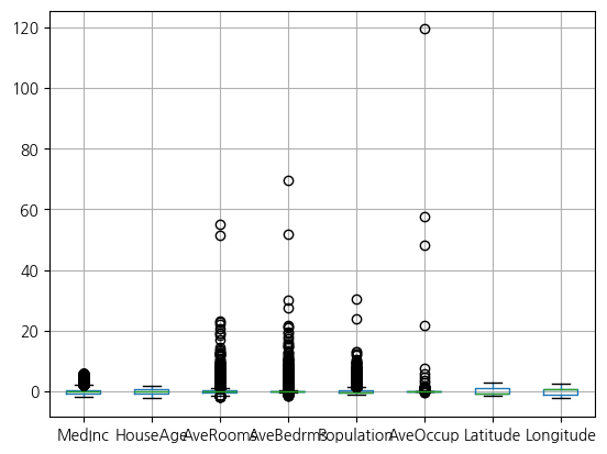

from sklearn.preprocessing import RobustScaler

scaler = RobustScaler()
scaled_data = scaler.fit_transform(housing.data)
# 중앙값이 0, IQR이 1인지 확인
assert np.allclose(np.median(scaled_data, axis=0), 0)
Q3, Q1 = np.percentile(scaled_data, [75, 25], axis=0)
assert np.allclose(Q3 - Q1, 1)
pd.DataFrame(scaled_data, columns=housing.data.columns).boxplot()
plt.ylim(-2, 2) # 이상치가 많아 y축 범위 제한
plt.show()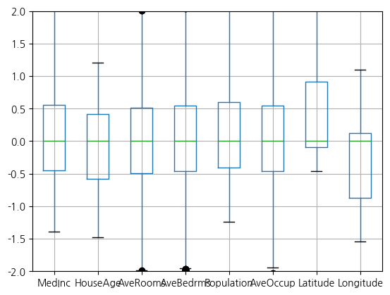

from sklearn.model_selection import train_test_split
from sklearn.neighbors import KNeighborsRegressor
from sklearn.linear_model import LinearRegression
from sklearn.preprocessing import MinMaxScaler
from sklearn.pipeline import make_pipeline

train_data, test_data, train_target, test_target = train_test_split(
    housing.data, housing.target, random_state=3)

model = LinearRegression()
model.fit(train_data, train_target)

scores = {}
scores['linear'] = {
    "train": model.score(train_data, train_target),
    "test": model.score(test_data, test_target)
}

model = KNeighborsRegressor(n_neighbors=1)
model = make_pipeline(MinMaxScaler(), model)
model.fit(train_data, train_target)
scores['knn'] = {
    "train": model.score(train_data, train_target),
    "test": model.score(test_data, test_target)
}

print(pd.DataFrame(scores).round(2))

       linear   knn
train    0.61  1.00
test     0.59  0.55

from sklearn.linear_model import LinearRegression
from sklearn.preprocessing import StandardScaler
from sklearn.pipeline import Pipeline, make_pipeline

# 단계명 미지정: 객체의 클래스 이름이 자동으로 단계명이 됨
model = make_pipeline(StandardScaler(), LinearRegression())
print(model.steps)

# 단계명 지정
model = Pipeline([
    ('scaler', StandardScaler()),
    ('linreg', LinearRegression())
])
print(model.steps)


model.fit(housing.data, housing.target)
# 매개변수 분석
특성별평균 = model.named_steps['scaler'].mean_
assert np.allclose(특성별평균, housing.data.mean())
w = model.named_steps['linreg'].coef_
b = model.named_steps['linreg'].intercept_
params = np.append(b, w)
pd.Series(params, index=['bias'] + list(housing.data.columns)).round(3)

[('standardscaler', StandardScaler()), ('linearregression', LinearRegression())]
[('scaler', StandardScaler()), ('linreg', LinearRegression())]

bias          2.069
MedInc        0.830
HouseAge      0.119
AveRooms     -0.266
AveBedrms     0.306
Population   -0.005
AveOccup     -0.039
Latitude     -0.900
Longitude    -0.871
dtype: float64

from sklearn.preprocessing import MinMaxScaler, StandardScaler, RobustScaler
from sklearn.linear_model import LinearRegression
from sklearn.pipeline import make_pipeline

scores = {}
model = make_pipeline(MinMaxScaler(), LinearRegression())
scores['minmax'] = 모델평가(model, housing.data, housing.target, random_state=3)
model = make_pipeline(StandardScaler(), LinearRegression())
scores['standard'] = 모델평가(model, housing.data, housing.target, random_state=3)
model = make_pipeline(RobustScaler(), LinearRegression())
scores['robust'] = 모델평가(model, housing.data, housing.target, random_state=3)
print(pd.DataFrame(scores).round(2))

       minmax  standard  robust
train    0.61      0.61    0.61
test     0.59      0.59    0.59

관찰: 선형 모델의 과소 적합

가설: 통계적 이상치들이 데이터의 복잡도를 증가시키는 것일 수도?

housing.data.describe().round(3)

from sklearn.preprocessing import StandardScaler, PolynomialFeatures
from sklearn.linear_model import LinearRegression

특성별필터 = {}
for 특성명 in housing.data.columns:
    특성열 = housing.data[특성명]
    Q3, Q1 = 특성열.quantile([0.75, 0.25])
    IRQ = Q3 - Q1 # Interquartile Range
    이상치하한 = Q1 - 1.5 * IRQ 
    이상치상한 = Q3 + 1.5 * IRQ
    특성별필터[특성명] = 특성열.between(이상치하한, 이상치상한)

model = make_pipeline(StandardScaler(), LinearRegression())

scores = {}
scores['all'] = 모델평가(model, housing.data, housing.target, random_state=3)

# 모든 필터의 교집합 
필터 = np.logical_and.reduce(list(특성별필터.values()))
print(len(housing.data), len(housing.data[필터]))
scores['filtered'] = 모델평가(
    model, housing.data[필터], housing.target[필터], random_state=3)

pd.DataFrame(scores).round(2)

20640 16842

1다항식 특성¶

선형 모델은 직선적인 관계만 표현하므로, 특성과 목표값의 관계가 곡선이면 과소적합하기 쉽습니다. 원래 특성의 거듭제곱( $x^2, x^3, \dots$ )을 새 특성으로 추가하면, 선형 모델이면서도 곡선 관계를 포착할 수 있습니다. PolynomialFeatures로 다항식 특성을 자동으로 만듭니다.

# 다항식 특성 추가
X2 = pd.concat([housing.data, housing.data**2], axis=1)
scores['poly'] = 모델평가(model, X2, housing.target, random_state=3)
scores['poly_filtered'] = 모델평가(model, X2[필터], housing.target[필터], random_state=3)

# 상호작용 특성 추가
model = make_pipeline(
    StandardScaler(), 
    PolynomialFeatures(degree=2, include_bias=False),
    LinearRegression())
scores['poly+interaction'] = 모델평가(model, housing.data, housing.target, random_state=3)
scores['poly+interaction_filtered'] = 모델평가(
    model, housing.data[필터], housing.target[필터], random_state=3)
# 3차항
model = make_pipeline(
    StandardScaler(), 
    PolynomialFeatures(degree=3, include_bias=False),
    LinearRegression())

scores['poly3'] = 모델평가(
    model, housing.data[필터], housing.target[필터], random_state=3)

pd.DataFrame(scores).round(2)

2상호 작용¶

$x = \left(x_1, x_2\right) \rightarrow x'=\left(x_1, x_2, x_1 x_2\right)$

두 특성을 곱한 항( $x_1 x_2$ )을 추가하면, 한 특성의 효과가 다른 특성의 값에 따라 달라지는 상호작용을 표현할 수 있습니다.

from sklearn.preprocessing import PolynomialFeatures
import scipy

특성수 = housing.data.shape[1]
# 상호 작용 (다항식 제외)
다항식차원확장기 = PolynomialFeatures(degree=2, include_bias=False, interaction_only=True)
X_interact = 다항식차원확장기.fit_transform(housing.data)
print(X_interact.shape)
특성조합수 = scipy.special.comb(특성수, 2, exact=True) # 조합의 가짓수
print(f'{특성수} + {특성조합수}')
assert X_interact.shape[1] == 특성수 + 특성조합수
print(다항식차원확장기.get_feature_names_out(housing.data.columns))

# 모든 2차 다항식: 다항식 + 상호작용
다항식차원확장기 = PolynomialFeatures(degree=2, include_bias=False)
X_poly = 다항식차원확장기.fit_transform(housing.data)
print(X_poly.shape)
특성조합수 = scipy.special.comb(특성수, 2, exact=True) # 중복조합의 가짓수
print(f'{특성수} + {특성수} + {특성조합수}')
assert X_poly.shape[1] == 특성수 * 2 + 특성조합수
print(다항식차원확장기.get_feature_names_out(housing.data.columns))

(20640, 36)
8 + 28
['MedInc' 'HouseAge' 'AveRooms' 'AveBedrms' 'Population' 'AveOccup'
 'Latitude' 'Longitude' 'MedInc HouseAge' 'MedInc AveRooms'
 'MedInc AveBedrms' 'MedInc Population' 'MedInc AveOccup'
 'MedInc Latitude' 'MedInc Longitude' 'HouseAge AveRooms'
 'HouseAge AveBedrms' 'HouseAge Population' 'HouseAge AveOccup'
 'HouseAge Latitude' 'HouseAge Longitude' 'AveRooms AveBedrms'
 'AveRooms Population' 'AveRooms AveOccup' 'AveRooms Latitude'
 'AveRooms Longitude' 'AveBedrms Population' 'AveBedrms AveOccup'
 'AveBedrms Latitude' 'AveBedrms Longitude' 'Population AveOccup'
 'Population Latitude' 'Population Longitude' 'AveOccup Latitude'
 'AveOccup Longitude' 'Latitude Longitude']
(20640, 44)
8 + 8 + 28
['MedInc' 'HouseAge' 'AveRooms' 'AveBedrms' 'Population' 'AveOccup'
 'Latitude' 'Longitude' 'MedInc^2' 'MedInc HouseAge' 'MedInc AveRooms'
 'MedInc AveBedrms' 'MedInc Population' 'MedInc AveOccup'
 'MedInc Latitude' 'MedInc Longitude' 'HouseAge^2' 'HouseAge AveRooms'
 'HouseAge AveBedrms' 'HouseAge Population' 'HouseAge AveOccup'
 'HouseAge Latitude' 'HouseAge Longitude' 'AveRooms^2'
 'AveRooms AveBedrms' 'AveRooms Population' 'AveRooms AveOccup'
 'AveRooms Latitude' 'AveRooms Longitude' 'AveBedrms^2'
 'AveBedrms Population' 'AveBedrms AveOccup' 'AveBedrms Latitude'
 'AveBedrms Longitude' 'Population^2' 'Population AveOccup'
 'Population Latitude' 'Population Longitude' 'AveOccup^2'
 'AveOccup Latitude' 'AveOccup Longitude' 'Latitude^2'
 'Latitude Longitude' 'Longitude^2']

3구간 분할 (이산화)¶

연속적인 특성을 몇 개의 구간(bin) 으로 나누어 범주형으로 바꾸는 것을 이산화라 합니다. 구간마다 다른 효과를 학습할 수 있어, 선형 모델로도 비선형 패턴을 일부 포착할 수 있습니다. KBinsDiscretizer로 구간 분할을 수행합니다.

from sklearn.preprocessing import KBinsDiscretizer

구간분할기 = KBinsDiscretizer(n_bins=4, encode='ordinal', strategy='uniform')
지역구간 = 구간분할기.fit_transform(housing.data[['Latitude', 'Longitude']])
# 구간별 도수
print(pd.DataFrame({
    '위도': pd.Series(지역구간[:, 0]).value_counts(),
    '경도': pd.Series(지역구간[:, 1]).value_counts()
}))
# 지역 경계 확인
위도경계, 경도경계 = 구간분할기.bin_edges_
pd.DataFrame({'위도': 위도경계, '경도': 경도경계}).round(2)

        위도     경도
0.0  11220   4917
1.0   2076   4161
2.0   6780  11203
3.0    564    359

from sklearn.preprocessing import StandardScaler, PolynomialFeatures
from sklearn.linear_model import LinearRegression
from sklearn.preprocessing import KBinsDiscretizer
from sklearn.pipeline import make_pipeline

구간분할기 = KBinsDiscretizer(n_bins=4, encode='ordinal', strategy='uniform')
지역구간 = 구간분할기.fit_transform(housing.data[['Latitude', 'Longitude']])
Xs = np.hstack([housing.data, 지역구간])

model = make_pipeline(
    StandardScaler(), 
    PolynomialFeatures(degree=3, include_bias=False),
    LinearRegression())

scores['poly3+location'] = 모델평가(
    model, Xs[필터], housing.target[필터], random_state=3)

pd.DataFrame(scores).round(2)

4알고리즘 비교¶

같은 캘리포니아 주택 데이터에 여러 회귀 알고리즘을 적용해 성능을 비교해 보겠습니다. 선형 모델, 거리 기반 kNN, 트리 앙상블을 같은 평가 흐름으로 견줍니다. 단위에 민감한 선형 모델과 kNN은 단위 변환을 함께 묶은 파이프라인으로 평가합니다.

from sklearn.linear_model import Ridge
from sklearn.neighbors import KNeighborsRegressor
from sklearn.ensemble import RandomForestRegressor
from sklearn.preprocessing import StandardScaler
from sklearn.pipeline import make_pipeline

모델들 = {
    '선형(릿지)': make_pipeline(StandardScaler(), Ridge()),
    'kNN': make_pipeline(StandardScaler(), KNeighborsRegressor()),
    '랜덤 포레스트': RandomForestRegressor(random_state=0),
}
점수 = {이름: 모델평가(model, housing.data, housing.target, random_state=4)
       for 이름, model in 모델들.items()}
pd.DataFrame(점수).T.round(3)

표에서 각 알고리즘의 훈련·시험 성능( $R^2$ )을 한눈에 비교할 수 있습니다. 선형 모델은 단순하고 해석하기 쉽지만 비선형 관계를 잘 담지 못하고, kNN과 랜덤 포레스트는 비선형 관계를 포착해 시험 성능이 더 높은 편입니다. 데이터에 어떤 알고리즘이 적합한지는 이렇게 여러 모델을 같은 기준으로 비교해 판단합니다.