로지스틱 회귀

import numpy as np
import pandas as pd
import matplotlib.pyplot as plt

random = np.random.default_rng(seed=0)

xs = np.linspace(0, 10, 100)
noise = random.normal(0, 1, size=xs.shape)
ys = 1.2 * xs + 3.4 + noise

Xs = np.stack([xs, ys], axis=1)
assert Xs.shape == (len(xs), 2)
labels = np.where(ys > ys - noise, 1, 0)


linear_model = lambda x, w, b: x @ w + b
params = random.normal(size=(3,))

sigmoid = lambda z: 1 / (1 + np.exp(-z))

outputs = linear_model(Xs, b=params[0], w=params[1:])
양성확률 = sigmoid(outputs)
예측 = np.where(양성확률 > 0.5, 1, 0)
정확도 = np.mean(예측 == labels)

print(f'b, w1, w2 = {params.round(3)} -> 정확도: {정확도:.1%}')
    
display(pd.DataFrame(Xs, columns=['x1', 'x2'])
        .assign(정답=labels)
        .assign(**{'p(y=1|x)': 양성확률})
        .assign(예측=예측)
        .head().round(3))

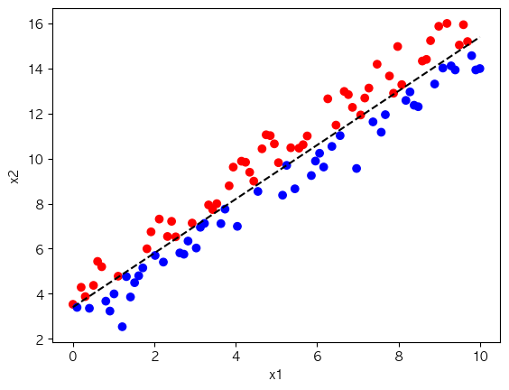
plt.scatter(Xs[:, 0], Xs[:, 1], c=labels, cmap='bwr')
plt.xlabel('x1'); plt.ylabel('x2')
plt.plot(xs, ys - noise, color='black', linestyle='--')
plt.show()

def 경사산출(X, y, p):
    표본수 = len(y)
    경사 = X.T @ (p - y)
    return 경사 / 표본수

linear_model = lambda x, w, b: x @ w + b

def 손실산출(y, p):
    delta = 1e-7
    p = np.clip(p, delta, 1 - delta)
    표본수 = len(y)
    손실 = - (y * np.log(p ) + (1 - y) * np.log(1 - p)).sum()
    return 손실 / 표본수

정확도평가 = lambda labels, z: (np.where(sigmoid(z) > 0.5, 1, 0) == labels).mean()

성능지표 = []

params = random.normal(size=(3,))
z = linear_model(Xs, b=params[0], w=params[1:])
성능지표.append({
    '손실': 손실산출(labels, sigmoid(z)),
    '정확도': 정확도평가(labels, z)
})

x0 = np.ones((len(Xs), 1))
경사 = [경사산출(np.hstack([x0, Xs]), labels, p=sigmoid(z))]
display(pd.DataFrame(
    경사, columns=['dL/db'] + [f'dL/dw{k+1}' for k in range(Xs.shape[1])]).round(3))

# 경사하강
학습률 = 1.0; 학습횟수 = 2000
param_history = [params]
for epoch in range(학습횟수):
    z = linear_model(Xs, b=params[0], w=params[1:])
    경사 = 경사산출(np.hstack([x0, Xs]), labels, p=sigmoid(z))
    params -= 학습률 * 경사
    param_history.append(params.copy())
    성능지표.append({
        '손실': 손실산출(labels, sigmoid(z)),
        '정확도': 정확도평가(labels, z)
    })

display(
    pd.concat([
        pd.DataFrame(param_history, columns=['b', 'w1', 'w2']),
        pd.DataFrame(성능지표),
    ], axis=1).round(3)
)

# Newton 방법 구현 (라인 서치 포함)
def hessian_계산(X, p):
    """
    로지스틱 회귀의 헤시안 행렬 계산
    H = (1/S) X^T D X, where D = diag(p(1-p))
    """
    표본수 = len(p)
    weights = p * (1 - p)
    weights = np.clip(weights, 1e-10, 1-1e-10)  # 수치 안정성
    weighted_X = X.T * weights
    hessian = weighted_X @ X
    return hessian / 표본수

def bce_loss(p, y, eps=1e-12):
    p = np.clip(p, eps, 1 - eps)
    return -np.mean(y * np.log(p) + (1 - y) * np.log(1 - p))

# Newton 방법 (라인 서치 포함)
params_newton = random.normal(size=(3,))
params_history_newton = [params_newton.copy()]
loss_history_newton = []

x0 = np.ones((len(Xs), 1))
X_aug = np.hstack([x0, Xs])

print("=" * 60)
print("Newton 방법 (2차 미분 + 라인 서치)")
print("=" * 60)

for epoch in range(100):
    # 현재 손실 및 그래디언트 계산
    z = Xs @ params_newton[1:] + params_newton[0]
    p = sigmoid(z)
    loss = bce_loss(p, labels)
    loss_history_newton.append(loss)
    
    if epoch % 10 == 0:
        print(f"에포크 {epoch:3d}: 손실 = {loss:.8f}")
    
    # 그래디언트
    gradient = 경사산출(X_aug, labels, p=p)
    
    # 헤시안 (2차 미분)
    hessian = hessian_계산(X_aug, p)
    
    # Newton 스텝 계산
    try:
        # 정규화된 헤시안 (수치 안정성)
        hessian_reg = hessian + 1e-6 * np.eye(hessian.shape[0])
        step_direction = np.linalg.solve(hessian_reg, gradient)
        
        # 라인 서치: step size α를 조정
        alpha = 1.0
        params_temp = params_newton - alpha * step_direction
        z_temp = Xs @ params_temp[1:] + params_temp[0]
        p_temp = sigmoid(z_temp)
        loss_temp = bce_loss(p_temp, labels)
        
        # 손실이 감소할 때까지 step size 감소
        max_ls_iter = 20
        for ls_iter in range(max_ls_iter):
            if loss_temp < loss:
                break
            alpha *= 0.5
            params_temp = params_newton - alpha * step_direction
            z_temp = Xs @ params_temp[1:] + params_temp[0]
            p_temp = sigmoid(z_temp)
            loss_temp = bce_loss(p_temp, labels)
        
        params_newton = params_temp
        params_history_newton.append(params_newton.copy())
        
        # 수렴 확인
        if np.linalg.norm(alpha * step_direction) < 1e-7:
            print(f"✓ 수렴 완료: {epoch}번 에포크")
            break
            
    except np.linalg.LinAlgError:
        print(f"경고: 선형 시스템 풀이 실패 (에포크 {epoch})")
        break

# 최종 정확도
z_newton = Xs @ params_newton[1:] + params_newton[0]
p_newton = sigmoid(z_newton)
정확도_newton = np.mean((p_newton > 0.5).astype(int) == labels)

print()
print("=" * 60)
print("수렴 방법 비교")
print("=" * 60)

비교_df = pd.DataFrame({
    '방법': ['경사 하강법 (1차)', 'Newton 방법 (2차)'],
    '에포크': [205, epoch + 1],
    'b': [params_optimized[0], params_newton[0]],
    'w1': [params_optimized[1], params_newton[1]],
    'w2': [params_optimized[2], params_newton[2]],
    '정확도': [정확도_개선, 정확도_newton]
})
display(비교_df.round(4))

print()
print(f"{'속도 향상':<30} {epoch+1 / 205 * 100:.1f}% (원래 경사하강 대비)")

# 손실 수렴 비교 시각화
fig, axes = plt.subplots(1, 2, figsize=(14, 5))

# 손실 곡선 비교
epochs_gd = np.arange(len(loss_history))
epochs_newton = np.arange(len(loss_history_newton))

axes[0].plot(epochs_gd, loss_history, 'o-', label='경사 하강법 (1차)', linewidth=2, markersize=4, alpha=0.7)
axes[0].plot(epochs_newton, loss_history_newton, 's-', label='Newton 방법 (2차)', linewidth=2, markersize=5, alpha=0.7)
axes[0].set_xlabel('에포크', fontsize=12)
axes[0].set_ylabel('손실', fontsize=12)
axes[0].set_title('손실 수렴 비교', fontsize=13, fontweight='bold')
axes[0].legend(fontsize=11)
axes[0].grid(True, alpha=0.3)
axes[0].set_yscale('log')

# 에포크 수 비교
methods = ['경사 하강법\n(1차 미분)', 'Newton\n(2차 미분)']
epochs_list = [205, epoch + 1]
colors = ['skyblue', 'lightcoral']
bars = axes[1].bar(methods, epochs_list, color=colors, edgecolor='black', linewidth=2)

# 바에 숫자 표시
for bar, ep in zip(bars, epochs_list):
    height = bar.get_height()
    axes[1].text(bar.get_x() + bar.get_width()/2., height,
                f'{int(ep)}',
                ha='center', va='bottom', fontsize=12, fontweight='bold')

axes[1].set_ylabel('필요한 에포크 수', fontsize=12)
axes[1].set_title('수렴 속도 비교', fontsize=13, fontweight='bold')
axes[1].grid(True, alpha=0.3, axis='y')
axes[1].set_ylim(0, 250)

plt.tight_layout()
plt.show()